Centroid-Coupled Formation Tracking
A consensus constraint at a coarse level can silently override tracking at the fine level, with every individual piece still behaving correctly.
Two rigid escort rings each track their own target. They are also tied to each other by a single centroid() edge one level up. That edge wins: both rings converge on the midpoint between the two targets and stay there, escorting neither – while each ring stays perfectly rigid and the solve stays exactly optimal for the specification as written.
The page also introduces two NestedSystems features with no equivalent in the flat Layered pipeline:
centroidrestriction maps – a subsystem can present the unweighted average of its members on an edge, not just one representative agent.approximation_gap– the energy cost of forcing a hierarchy to stay rigid, measured against an unconstrained baseline.
Topology
ringA (4 agents) and ringB (5 agents) sit under one subsystem, mid. The sizes differ deliberately: the rings end up on top of each other, and this keeps them distinguishable.
mid's internal edge uses centroid() at both ends, tying ringA's average position to ringB's rather than to any single agent. Because mid is a single vertex at the coarsest level, this is not a soft preference – it defines which configurations of mid are admissible. The two centroids are forced to coincide.
Pinning each ring to its target
Each ring observes its own target through several agents at once – every other agent around the ring – rather than through the usual single representative. redundant_pin splits the work: the first pin is a plain project(1), and every pin after it is a translation_pin.
That distinction matters. Several full pins to one target are mutually inconsistent for a rigid body by construction, and the inconsistency is the point: spread across the ring as a least-squares compromise, it rebalances the ring's "vote" against competing edges elsewhere in the tower (n_ring_formation.jl is where that pays off).
But the compromise does not stay confined to translation. It also drags the affine homogeneous coordinate away from 1, and these restriction maps represent pure translation only while that row is exactly 1 – so the whole rigid body silently rescales. translation_pin pins the translation components alone and leaves that row untouched.
There is a useful side effect. translation_pin is deferred – like centroid(), it has no single representative vertex at the finest level – so only the one project(1) pin per ring reaches the direct baseline below. solve_direct therefore reduces to the same "two independent rigid rings, zero energy" case a plain single-pin design would give, and the redundancy does not muddy the comparison.
What to watch
The hierarchical solve cannot place ringA on target 1 and ringB on target 2 independently. It must find the one shared point that best satisfies both pins at once, and that point is exactly the midpoint of the two targets (verified numerically below).
As the targets spiral apart, both rings sit together on that midpoint while their own targets recede in opposite directions. The gap panel quantifies what this costs; the tracking-error panel shows the failure directly, growing with separation instead of settling to zero.
using CellularSheaves
using CellularSheaves.ControlSheaves.NestedSystems
using CellularSheaves.ControlSheaves.NestedDSL
using CellularSheaves.ControlSheaves.AgentControllers
using LinearAlgebra
using Plots
using Printf

# Located from the package root, not `@__DIR__`: while Literate.jl executes a page, `@__DIR__`
# points at the *output* directory rather than at this file. The simulation driver and the
# multi-pin helpers live in `NestedSystems`, already loaded above.
include(joinpath(pkgdir(CellularSheaves), "docs", "literate", "nested", "_plot_helpers.jl"))Main.var"##3123".fade_alphaTopology specification
const D = 4   # SE(3) homogeneous: 3D translation + 1 homogeneous row
const M_A, M_B = 4, 5

# Written in the `NestedDSL` language. `@nested_system` *runs* its block, so the pin
# loops below are ordinary Julia `for` loops rather than DSL constructs, and `via(...)` presents
# an arbitrary `RestrictionSpec` -- here `redundant_pin` -- on an edge.
topology = @nested_system begin
    @dim D
    @system mid begin
        @team ringA = ring(M_A; radius=1.0)
        @team ringB = ring(M_B; radius=1.0)
        @link centroid(ringA) => centroid(ringB)
    end
    @target t1 t2
    for k in 1:2:M_A
        @observe via(mid.ringA, redundant_pin(M_A, D, k)) => t1
    end
    for k in 1:2:M_B
        @observe via(mid.ringB, redundant_pin(M_B, D, k)) => t2
    end
end
SystemFragment(9 terms: 0 team, 1 system, 0 link, 2 target, 5 observe)Target motion: two targets spiraling apart
Both targets orbit a common centre at rate ω, while their shared radius ρ(t) = ρ0 + k t grows. Their separation Δ(t) = 2ρ(t) therefore widens smoothly, sweeping the demonstration from a small gap to a clearly growing one within a single run.
The velocities and accelerations below are exact analytic derivatives (the polar product rule), checked against finite differences beforehand rather than finite-differenced at runtime.
const ρ0, k_sep, ω, h_alt = 0.5, 0.15, 0.4, 1.5

ρ(t) = ρ0 + k_sep * t
θ(t) = ω * t

target1(t) = [ρ(t) * cos(θ(t)), ρ(t) * sin(θ(t)), h_alt, 1.0]
target1_vel(t) = [k_sep * cos(θ(t)) - ρ(t) * ω * sin(θ(t)),
                  k_sep * sin(θ(t)) + ρ(t) * ω * cos(θ(t)), 0.0, 0.0]
target1_acc(t) = [-2k_sep * ω * sin(θ(t)) - ρ(t) * ω^2 * cos(θ(t)),
                    2k_sep * ω * cos(θ(t)) - ρ(t) * ω^2 * sin(θ(t)), 0.0, 0.0]

# target2 sits diametrically opposite target1 (angle θ+π): negate x, y and their derivatives.
target2(t) = [-target1(t)[1], -target1(t)[2], h_alt, 1.0]
target2_vel(t) = [-target1_vel(t)[1], -target1_vel(t)[2], 0.0, 0.0]
target2_acc(t) = [-target1_acc(t)[1], -target1_acc(t)[2], 0.0, 0.0]
target2_acc (generic function with 1 method)Dynamics and gains
DT, STEPS = 0.05, 200
dyn = QuadrotorDynamics()
Ad, Bd = CellularSheaves.AgentControllers.discrete_matrices(dyn, DT)
Q_lqr = Matrix(Diagonal([500.0, 500.0, 500.0, 150.0, 150.0, 100.0, 100.0, 100.0, 5.0, 5.0]))
R_lqr = Matrix(Diagonal([0.005, 0.005, 0.005]))
K = CellularSheaves.AgentControllers.solve_dare(Ad, Bd, 10 * Q_lqr, R_lqr)
3×10 Matrix{Float64}:
0.0 0.0 21.1663 0.0 0.0 0.0 0.0 10.5247 0.0 0.0
0.0 -1.46672 0.0 2.39234 0.0 0.0 -1.07034 0.0 0.255508 0.0
1.46672 0.0 0.0 0.0 2.39234 1.07034 0.0 0.0 0.0 0.255508The dynamics binding is written in the same language, but as a separate fragment merged onto the topology above. It has to be: the gain K does not exist until solve_dare runs, and that is ordinary Julia which must come first. Because a fragment is a first-class value, one specification can be assembled from pieces written wherever they belong.
system = compile_nested_system(merge(topology, @nested_system begin
    @bind dynamics=dyn K_lqr=K
end))
spec, tower, bindings = system.spec, system.tower, system.bindings

# Agent index blocks, looked up by name rather than reconstructed by hand from team sizes.
ring_ranges = [agent_range(system, "mid.ringA"), agent_range(system, "mid.ringB")]
2-element Vector{UnitRange{Int64}}:
1:4
5:9Run the closed-loop simulation with full feedforward
prob = NestedEscortProblem(tower, bindings, [target1, target2];
                           target_velocities=[target1_vel, target2_vel],
                           target_accelerations=[target1_acc, target2_acc],
                           dt=DT, steps=STEPS)
res = run_nested_escort_simulation(prob; use_feedforward=true)
time_grid = 0:DT:(STEPS*DT)0.0:0.05:10.0Diagnostics: formation error, tracking error, and the approximation gap
approximation_gap needs no agent dynamics at all – it is a static property of the tower and the current target positions – so it is swept separately from the closed-loop simulation above, at the same time grid.
gap_history = [approximation_gap(tower, [target1(t), target2(t)]) for t in time_grid[1:STEPS]]

ring_names = ["ringA", "ringB"]
ring_radius = [1.0, 1.0]
ring_targets = [target1, target2]
form_err = [zeros(STEPS) for _ in 1:2]
track_err = [zeros(STEPS) for _ in 1:2]

for step in 1:STEPS
    t = time_grid[step]
    for (r, rng) in enumerate(ring_ranges)
        positions = [res.sim_data[step][i][1:3] for i in rng]
        c = sum(positions) / length(positions)
        form_err[r][step] = sum(abs(norm(p .- c) - ring_radius[r]) for p in positions) / length(positions)
        track_err[r][step] = norm(c[1:2] .- ring_targets[r](t)[1:2])
    end
end
Plots
colors = [:steelblue, :crimson]

# Panel 1: top-down view, and the animated version below both need consistent axis limits --
# computed once, from every agent and target position across the whole run.
all_x = Float64[]; all_y = Float64[]
for rng in ring_ranges, i in rng, step in 1:STEPS
    push!(all_x, res.sim_data[step][i][1]); push!(all_y, res.sim_data[step][i][2])
end
for traj in (target1, target2), t in time_grid[1:STEPS]
    p = traj(t)
    push!(all_x, p[1]); push!(all_y, p[2])
end
const TOPDOWN_XLIM = (minimum(all_x) - 0.5, maximum(all_x) + 0.5)
const TOPDOWN_YLIM = (minimum(all_y) - 0.5, maximum(all_y) + 0.5)

# Panel 1 proper: a composite of the *whole* run, not just its final state. Agent paths are drawn
# thin and faint, so overlapping low-alpha paths darken where several agents pass through the
# same region -- which is what makes the two rings' shared convergence on the midpoint visible.
# Ring outlines are drawn at a few evenly spaced snapshots, fading faint (early) to solid (final).
function top_down_composite(; n_snapshots::Int=8)
    snaps = snapshot_steps(STEPS, n_snapshots)
    p = plot(title="Top-Down View (full trajectory)", aspect_ratio=1,
            xlabel="x (m)", ylabel="y (m)", xlims=TOPDOWN_XLIM, ylims=TOPDOWN_YLIM,
            legend=:topright, size=(600, 500))
    for (r, rng) in enumerate(ring_ranges)
        for i in rng
            px = [res.sim_data[s][i][1] for s in 1:STEPS]
            py = [res.sim_data[s][i][2] for s in 1:STEPS]
            plot!(p, px, py, color=colors[r], alpha=0.12, linewidth=1, label="")
        end
        for (si, s) in enumerate(snaps)
            a = fade_alpha(si, length(snaps))
            fx = [res.sim_data[s][i][1] for i in rng]
            fy = [res.sim_data[s][i][2] for i in rng]
            plot!(p, [fx; fx[1]], [fy; fy[1]], color=colors[r], linestyle=:dash, alpha=a,
                 label=(s == snaps[end] ? ring_names[r] : ""))
            scatter!(p, fx, fy, color=colors[r], markersize=3, alpha=a, label="")
        end
    end
    for (r, traj) in enumerate([target1, target2])
        tp = [traj(t) for t in time_grid[1:STEPS]]
        plot!(p, [q[1] for q in tp], [q[2] for q in tp], color=colors[r], linestyle=:dot, alpha=0.5, label="")
        for (si, s) in enumerate(snaps)
            pt = traj(time_grid[s])
            a = fade_alpha(si, length(snaps))
            scatter!(p, [pt[1]], [pt[2]], marker=:star5, markersize=(s == snaps[end] ? 10 : 5),
                    color=colors[r], alpha=a, label=(s == snaps[end] ? "target $r" : ""))
        end
    end

    # The midpoint of the two targets -- direct visual proof that the rings are converging on
    # this shared point rather than on either target.
    mp = [(target1(t) .+ target2(t)) ./ 2 for t in time_grid[1:STEPS]]
    plot!(p, [q[1] for q in mp], [q[2] for q in mp], color=:black, linestyle=:dot, alpha=0.4, label="")
    scatter!(p, [mp[end][1]], [mp[end][2]], marker=:xcross, markersize=8, color=:black,
            label="target midpoint")
    return p
end

p1 = top_down_composite()

# The animation reuses the same per-step rendering in miniature: current positions and outline
# only, no accumulated trail. Its job is to convey motion; panel 1 already shows the whole run.
function top_down_frame(step::Int)
    t = time_grid[step]
    p = plot(title=@sprintf("Top-Down View (t = %.2f s)", t), aspect_ratio=1,
            xlabel="x (m)", ylabel="y (m)", xlims=TOPDOWN_XLIM, ylims=TOPDOWN_YLIM,
            legend=:topright, size=(600, 500))
    for (r, rng) in enumerate(ring_ranges)
        cx = [sum(res.sim_data[s][i][1] for i in rng) / length(rng) for s in 1:step]
        cy = [sum(res.sim_data[s][i][2] for i in rng) / length(rng) for s in 1:step]
        plot!(p, cx, cy, color=colors[r], alpha=0.4, label="")

        fx = [res.sim_data[step][i][1] for i in rng]
        fy = [res.sim_data[step][i][2] for i in rng]
        scatter!(p, fx, fy, color=colors[r], markersize=4, label=ring_names[r])
        plot!(p, [fx; fx[1]], [fy; fy[1]], color=colors[r], linestyle=:dash, label="")
    end
    for (r, traj) in enumerate([target1, target2])
        tp = [traj(tt) for tt in time_grid[1:step]]
        plot!(p, [q[1] for q in tp], [q[2] for q in tp], color=colors[r], linestyle=:dot, alpha=0.5, label="")
        pt = traj(t)
        scatter!(p, [pt[1]], [pt[2]], marker=:star5, markersize=10, color=colors[r], label="target $r")
    end

    # The midpoint of the two targets -- direct visual proof that the rings are converging on
    # this shared point rather than on either target.
    mp = [(target1(tt) .+ target2(tt)) ./ 2 for tt in time_grid[1:step]]
    plot!(p, [q[1] for q in mp], [q[2] for q in mp], color=:black, linestyle=:dot, alpha=0.4, label="")
    scatter!(p, [mp[end][1]], [mp[end][2]], marker=:xcross, markersize=8, color=:black,
            label="target midpoint")
    return p
end

# Panel 2: formation radius error over time.
p2 = plot(title="Formation Radius Error", xlabel="time (s)", ylabel="error (m)")
for r in 1:2
    plot!(p2, time_grid[1:STEPS], form_err[r], color=colors[r], label=ring_names[r], linewidth=2)
end

# Panel 3: centroid tracking error over time.
p3 = plot(title="Centroid Tracking Error", xlabel="time (s)", ylabel="error (m)")
for r in 1:2
    plot!(p3, time_grid[1:STEPS], track_err[r], color=colors[r], label=ring_names[r], linewidth=2)
end

# Panel 4: the approximation gap -- what the hierarchy's rigidity costs, over time.
p4 = plot(title="Hierarchical vs. Direct Energy", xlabel="time (s)", ylabel="Dirichlet energy")
plot!(p4, time_grid[1:STEPS], [g.hierarchical for g in gap_history], color=:darkorange,
     label="hierarchical", linewidth=2)
plot!(p4, time_grid[1:STEPS], [g.direct for g in gap_history], color=:gray, label="direct",
     linewidth=2, linestyle=:dash)
plot!(p4, time_grid[1:STEPS], [g.gap for g in gap_history], color=:forestgreen, label="gap",
     linewidth=2, linestyle=:dot)

plot(p1, p2, p3, p4, layout=(2, 2), size=(1000, 800),
    plot_title="Centroid-Coupled Formation: Gap Opens as Targets Separate")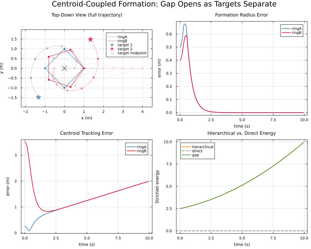
direct stays roughly flat. It reflects only the cost of pinning several points of one rigid ring to a single target at once – unavoidable as soon as more than one agent observes the same point – and that cost does not depend on how far apart the two targets are.
hierarchical and gap both climb above that floor as the separation grows. The difference is exactly what it costs to force ringA and ringB onto one shared point while their targets pull apart.
@printf("Final gap: %.4f  (hierarchical: %.4f, direct: %.4f)\n",
       gap_history[end].gap, gap_history[end].hierarchical, gap_history[end].direct)
Final gap: 9.9401 (hierarchical: 9.9401, direct: 0.0000)
Animated top-down view
Same top_down_frame function as panel 1 above, stepped through the run.
anim = @animate for step in 1:4:STEPS
    top_down_frame(step)
end
gif(anim, "centroid_formation_top_down.gif", fps=10)
Plots.AnimatedGif("/home/runner/work/CellularSheaves.jl/CellularSheaves.jl/docs/src/generated/nested/centroid_formation_top_down.gif")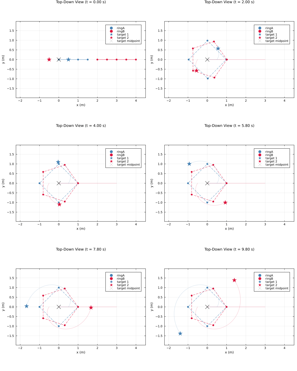
println("Centroid formation tracking example complete.")Centroid formation tracking example complete.